Busiest air routes
Introduction
This is a simple exercise to extract data from a Wikipedia page (List of busiest passenger air routes) and performing a basic data visualisation.
Why am I doing this? I somehow really got into aviation in the past 2 years. Due to the COVID travel restriction, I have spent days on YouTube watching planes taking off and landing. In a moment of self-indulgence, I would also like to add that Airbus 380 is such a beautiful engineering marvel and it is sad that COVID fastened the end of its production.
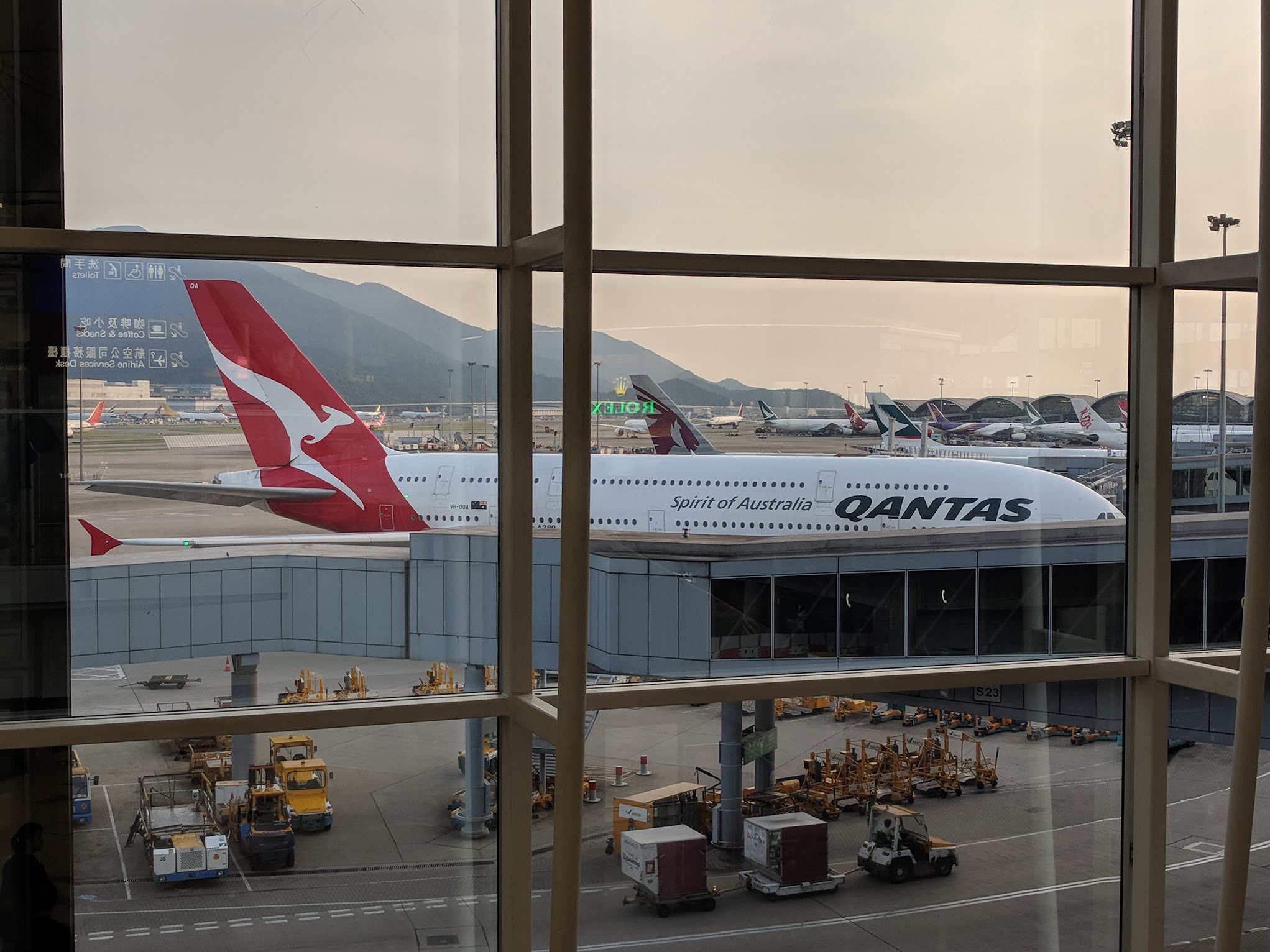
Airbus 380 at Hong Kong airport, 2018
Extracting data
We can, in theory, copy and paste the data to an Excel sheet and then import the data. However, we will try to do something a bit fancier and use the rvest package to extract this data.
The only downside with extracting the data in this way is that if the webpage is updated, then our code might not work. Hence, I will also save a copy of this data in my GitHub.
suppressPackageStartupMessages({
  library(xml2)
  library(rvest)
  library(tidyverse)
})
webpage = xml2::read_html("https://en.wikipedia.org/wiki/List_of_busiest_passenger_air_routes")
raw_tbl = webpage %>%
html_element("table") %>%
html_table()
raw_tbl## # A tibble: 50 x 7
## Rank `Airport 1` `Airport 2` `Distance (km)` `2018[1]` `2017[2]` Type
## <int> <chr> <chr> <int> <chr> <chr> <chr>
## 1 1 Jeju Seoul-Gimpo 449 14,107,4… 13,460,3… Domest…
## 2 2 Sapporo Tokyo-Haneda 835 9,698,639 8,726,502 Domest…
## 3 3 Sydney Melbourne 705 9,245,392 9,090,941 Domest…
## 4 4 Fukuoka Tokyo-Haneda 889 8,762,547 7,864,000 Domest…
## 5 5 Mumbai Delhi 1150 7,392,155 7,129,943 Domest…
## 6 6 Hanoi Ho Chi Minh C… 1171 6,867,114 6,769,823 Domest…
## 7 7 Beijing Shanghai-Hong… 1081 6,518,997 6,833,684 Domest…
## 8 8 Hong Kong Taipei-Taoyuan 802 6,476,268 6,719,030 Intern…
## 9 9 Tokyo-Haneda Naha 1573 5,829,712 5,269,481 Domest…
## 10 10 Jakarta Surabaya 700 5,649,046 5,271,304 Domest…
## # … with 40 more rows## We are only interested in the 2018 passenger numbers
subset_tbl = raw_tbl %>%
dplyr::transmute(
rank = Rank,
airport1 = `Airport 1`,
airport2 = `Airport 2`,
distance = `Distance (km)`,
passengers = `2018[1]` %>% str_remove_all(",") %>% as.integer(),
type = Type)
subset_tbl## # A tibble: 50 x 6
## rank airport1 airport2 distance passengers type
## <int> <chr> <chr> <int> <int> <chr>
## 1 1 Jeju Seoul-Gimpo 449 14107414 Domestic
## 2 2 Sapporo Tokyo-Haneda 835 9698639 Domestic
## 3 3 Sydney Melbourne 705 9245392 Domestic
## 4 4 Fukuoka Tokyo-Haneda 889 8762547 Domestic
## 5 5 Mumbai Delhi 1150 7392155 Domestic
## 6 6 Hanoi Ho Chi Minh City 1171 6867114 Domestic
## 7 7 Beijing Shanghai-Hongqiao 1081 6518997 Domestic
## 8 8 Hong Kong Taipei-Taoyuan 802 6476268 International
## 9 9 Tokyo-Haneda Naha 1573 5829712 Domestic
## 10 10 Jakarta Surabaya 700 5649046 Domestic
## # … with 40 more rowswrite_csv(x = subset_tbl, file = "raw_airports_data.csv")Notice that most of the “airports” are actually just the name of the city. We will use this to grab the longitude and latitude information. However, there are some exceptions like “Tokyo-Haneda”, where “Haneda” is one of the two international airports in the city of Tokyo. We will need to clean up these exceptions for consistency.
clean_tbl = subset_tbl %>%
  dplyr::mutate(
    city1 = purrr::map_chr(.x = airport1,
                       .f = ~ str_split(.x, "-")[[1]][1]),
    city2 = purrr::map_chr(.x = airport2,
                       .f = ~ str_split(.x, "-")[[1]][1]))

clean_tbl
## # A tibble: 50 x 8
## rank airport1 airport2 distance passengers type city1 city2
## <int> <chr> <chr> <int> <int> <chr> <chr> <chr>
## 1 1 Jeju Seoul-Gimpo 449 14107414 Domestic Jeju Seoul
## 2 2 Sapporo Tokyo-Haneda 835 9698639 Domestic Sapporo Tokyo
## 3 3 Sydney Melbourne 705 9245392 Domestic Sydney Melbourne
## 4 4 Fukuoka Tokyo-Haneda 889 8762547 Domestic Fukuoka Tokyo
## 5 5 Mumbai Delhi 1150 7392155 Domestic Mumbai Delhi
## 6 6 Hanoi Ho Chi Minh… 1171 6867114 Domestic Hanoi Ho Chi M…
## 7 7 Beijing Shanghai-Ho… 1081 6518997 Domestic Beijing Shanghai
## 8 8 Hong Kong Taipei-Taoy… 802 6476268 Internat… Hong K… Taipei
## 9 9 Tokyo-Han… Naha 1573 5829712 Domestic Tokyo Naha
## 10 10 Jakarta Surabaya 700 5649046 Domestic Jakarta Surabaya
## # … with 40 more rowsGetting locations for the cities
Google Maps API
There are many ways of getting the location information for cities. In the past, I have found the most reliable way is to get it through ggmap which uses the Google Maps API, but this means you must set up a Google Cloud Platform billing account with them (which unfortunately requires a credit card). See this documentation. Once a project is set up with the Google Cloud Platform, you will then need to enable the Google Maps API by searching for it in the top search bar. The API key is required too, see the documentations for ggmap::register_google for more information.
Aside: is all these worth it? In my experience, absolutely! Because Google Maps is very smart and tends to understand certain complexities that you didn’t think of and handle those for you. For example, if you are interested in the city of Sydney, Google Maps will understand that to be the city of Sydney in Australia, not the city in Nova Scotia, Canada (I don’t know how they do this, but my guess is that they will return results that are more relevant, because, well, they are Google). Google Cloud is also offering free credits for most of their basic services, so one can take advantage of these without incurring substantial costs.
To ensure code reproducibility, I will use the code below to download the coordinates for all the cities, save it as a CSV and make it available on GitHub.
library(ggmap)
# ggmap::geocode("Sydney, Australia", output = "latlon", source = "google")
all_cities = c(clean_tbl$city1, clean_tbl$city2) %>% unique
all_geocode = ggmap::geocode(location = all_cities, output = "latlon")
city_tbl = tibble(
  city = all_cities,
  lon = all_geocode$lon,
  lat = all_geocode$lat)

readr::write_csv(x = city_tbl, file = "./city_tbl.csv")
Alternatively, if you don’t want to register for Google’s billings, you could use the tidygeocoder’s geocode function to get the latitude/longitude information via Open Street Map, which doesn’t require registration, but in my experience, it can be slower than Google Maps.
tidygeocoder location extractions
A small example:
city_tbl = tibble(
  city = c(clean_tbl$city1, clean_tbl$city2) %>% unique) %>%
  tidygeocoder::geocode(city, method = 'osm', lat = latitude , long = longitude)
Simple maps location extractions
You could also use the data provided in https://simplemaps.com/data/world-cities to perform data joins to get the location information. The downloaded data looks quite tidy with additional ASCII encoding and I was quite impressed with the quality of the data.
Joining data and visualise
Once we have the location information we can simply join the data as followed:
city_tbl = readr::read_csv(file = "https://gist.githubusercontent.com/kevinwang09/006d00ee7a43778171e7fc2fd409cdd6/raw/f12ec9deecdd99b093d0c819e21b125a7f7d4afd/city_tbl.csv")##
## ── Column specification ────────────────────────────────────────────────────────
## cols(
## city = col_character(),
## lon = col_double(),
## lat = col_double()
## )joined_data = clean_tbl %>%
left_join(city_tbl, by = c("city1" = "city")) %>%
left_join(city_tbl, by = c("city2" = "city"), suffix = c("1", "2"))I really like plotly’s globe visualisation, because you can click and drag the globe, which is really nice.
Using this visualisation, we can see most of the busiest routes in the world are concentrated around Asia. What surprised me a few years ago is that Australia, despite its small population, also had a couple of routes made it to this list, with Sydney - Melbourne being the third on the list. In my experience, on a good day, there could be two planes at the Sydney airport flying to Melbourne but only 10 minutes apart. Which I must admit was a rare luxury that I never realised.
library(plotly)##
## Attaching package: 'plotly'## The following object is masked from 'package:ggplot2':
##
## last_plot## The following object is masked from 'package:stats':
##
## filter## The following object is masked from 'package:graphics':
##
## layoutgeo <- list(
scope = 'world',
projection = list(type = 'orthographic'),
showland = TRUE,
landcolor = toRGB("gray95"),
countrycolor = toRGB("gray80")
)
fig <- plot_geo(color = I("red"))
fig <- fig %>%
add_markers(
data = joined_data, x = ~lon1, y = ~lat1, text = ~city1,
hoverinfo = "text", alpha = 0.5) %>%
add_markers(
data = joined_data, x = ~lon2, y = ~lat2, text = ~city2,
hoverinfo = "text", alpha = 0.5) %>%
add_segments(
data = group_by(joined_data, rank),
x = ~lon1, xend = ~lon2,
y = ~lat1, yend = ~lat2,
alpha = 0.3, size = I(1),
hoverinfo = "none") %>%
layout(
title = 'Busiest air routes in the world',
geo = geo,
showlegend = FALSE,
height = 800)
fig